Cleaning up and interpreting real staging: a worked example with mrpheus • hypnoR

library(hypnoR)

This picks up exactly where mrpheus’s sleep-staging-demo article leaves off: staging is done, and the resulting tibble is ready to hand to hypnoR. What follows is the actual process of turning that raw staging into something you’d trust for cycle counts and architecture metrics – including a couple of dead ends, because they’re informative.

Getting the data in

staging <- readRDS(system.file("extdata", "SC4001E0_staging.rds", package = "mrpheus"))

mrp_hyp <- mrpheus::export_hypnogram(
  staging,
  epoch_s        = 30,
  start_time     = as.POSIXct("2024-01-01 16:13:00", tz = "UTC"),
  participant_id = "SC4001"
)
#> ✔ Hypnogram ready: 2650 epochs. Pass to `hypnor::new_hypnogram()` once hypnor is available.

hyp <- new_hypnogram(mrp_hyp)

First look: a lot of REM, in odd places

plot_hypnogram(hyp)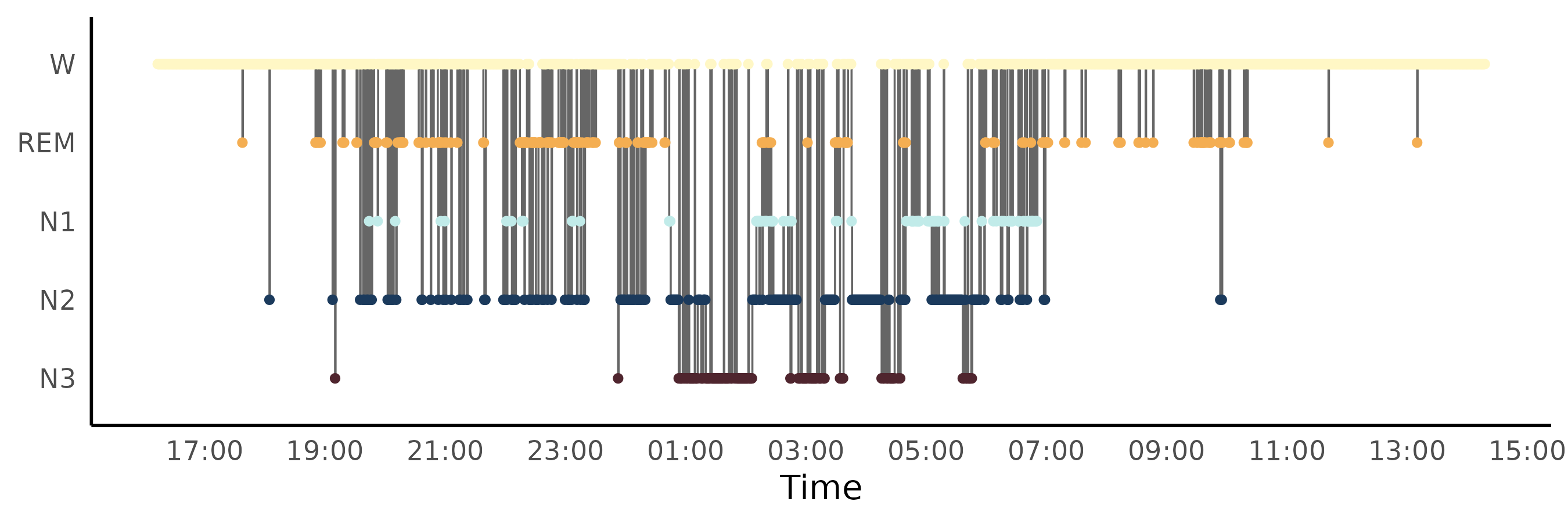

Two things jump out. First, REM appears scattered across nearly the whole 22-hour recording, including well into what should be plain daytime Wake. Second, the trace looks a lot busier than the smooth textbook hypnograms you’re used to seeing.

Is this a bug?

Worth checking rather than assuming either way. mrpheus::stage_epochs()’s entire staging decision is:

stage <- stage_labels[apply(probs, 1, which.max)]

A pure per-epoch argmax over the LightGBM posteriors, with no temporal smoothing or continuity constraint. That’s not a mrpheus bug – it’s how the underlying YASA-parity classifier is designed to work, and YASA itself doesn’t smooth by default either. So isolated single-epoch flips are expected precisely where the model is genuinely uncertain, not a sign of something broken.

That’s a hypothesis, though, not a conclusion. staging carries the posterior probabilities, so it’s checkable directly: are the scattered REM epochs concentrated among low-confidence calls?

rl <- rle(staging$stage)
staging$run_id     <- rep(seq_along(rl$lengths), rl$lengths)
run_lengths         <- aggregate(epoch ~ run_id, staging, length)
staging$run_length <- run_lengths$epoch[match(staging$run_id, run_lengths$run_id)]
staging$confidence <- pmax(staging$prob_W, staging$prob_N1, staging$prob_N2,
                           staging$prob_N3, staging$prob_REM)

isolated_rem  <- staging$confidence[staging$stage == "REM" & staging$run_length == 1]
sustained_rem <- staging$confidence[staging$stage == "REM" & staging$run_length >= 5]

summary(isolated_rem)
#>    Min. 1st Qu.  Median    Mean 3rd Qu.    Max. 
#>  0.2751  0.3972  0.4441  0.4632  0.5059  0.8922
summary(sustained_rem)
#>    Min. 1st Qu.  Median    Mean 3rd Qu.    Max. 
#>  0.3295  0.4481  0.5408  0.5720  0.6814  0.8640

Isolated single-epoch REM calls carry meaningfully lower confidence than REM epochs that are part of a sustained, multi-minute run. That’s consistent with “genuine borderline calls,” not a processing error – N1/REM is a well-known confusion pair for automatic staging, since both look comparatively wake-like on EEG and are mainly told apart by EMG atonia and EOG, which are noisier signals.

Smoothing

Confirmed-as-expected doesn’t mean desirable for downstream analysis, though. A single-epoch REM blip during otherwise clear NREM sleep is usually implausible even when the classifier briefly favoured it, and it’s worth cleaning up before cycle detection sees it.

hyp_smooth <- smooth_hypnogram(hyp, method = c("aasm_isolated", "min_run"), min_run_epochs = 4)
mean(hyp_smooth$stage != hyp_smooth$stage_raw)
#> [1] 0.1283019

Worth checking what’s actually left rather than assuming smoothing solved everything:

rl_smooth <- rle(as.character(hyp_smooth$stage))
table(rl_smooth$lengths[rl_smooth$values == "REM"])
#> 
#>  1  2  3  4  6  7  9 10 12 13 14 17 
#>  1  2  1  3  1  6  1  1  1  1  2  2

Most of the remaining REM runs are 3.5-8.5 minutes long – individually plausible REM bout durations, not noise. There are simply more separate REM excursions across the night than one ultradian cycle count would predict. Pushing min_run_epochs higher from here would mean deleting real multi-minute REM bouts to force the count down, which is the wrong lever to pull. compute_cycles(method = "aasm")’s gap-tolerance exists for exactly this situation – fragmented REM separated by brief interruptions that shouldn’t count as separate cycles:

nrow(compute_cycles(hyp_smooth, method = "aasm"))
#> [1] 10

Still high. The remaining explanation: some of those REM excursions are sitting out in daytime Wake, far from the main nocturnal cluster, each getting counted as its own “cycle” simply because nothing else is nearby.

Windowing: isolating the real sleep period

SC4001 is a 22-hour ambulatory recording – most of it is ordinary daytime Wake before and after the one real sleep opportunity. window_hypnogram() restricts analysis to just the sleep period. The data-driven version (first sleep epoch to last sleep epoch) is more reliable here than borrowing an illustrative epoch range from a plotting example, since a plot-oriented slice isn’t guaranteed to land exactly on the true sleep offset:

sleep_idx    <- which(as.character(hyp_smooth$stage) != "W")
onset_epoch  <- hyp_smooth$epoch[sleep_idx[1]]
offset_epoch <- hyp_smooth$epoch[sleep_idx[length(sleep_idx)]]
(offset_epoch - onset_epoch + 1) * 30 / 3600  # duration in hours -- sanity check
#> [1] 15.48333

hyp_sleep <- window_hypnogram(hyp_smooth, from_epoch = onset_epoch, to_epoch = offset_epoch)
nrow(compute_cycles(hyp_sleep, method = "aasm"))
#> [1] 10

A duration in the expected 7-8 hour range, and a cycle count that now sits in a physiologically ordinary range – confirming the earlier inflated count really was a daytime-Wake artifact of analysing the whole recording, not something smoothing could have fixed.

Comparing cycle-detection methods

With a properly windowed hypnogram, it’s worth seeing how much "aasm"’s gap-tolerance actually changes versus the strict "feinberg_floyd" method:

cyc_ff   <- compute_cycles(hyp_sleep, method = "feinberg_floyd")
cyc_aasm <- compute_cycles(hyp_sleep, method = "aasm")

nrow(cyc_ff)
#> [1] 15
nrow(cyc_aasm)
#> [1] 10

feinberg_floyd (no interruption tolerance) tends to fragment more aggressively than aasm (tolerates brief non-REM interruptions up to rem_gap_min minutes) – which method is “right” depends on whether a brief arousal mid-REM should end that REM period or not, a genuinely debatable scoring choice rather than a settled fact.

Both plotting styles, side by side

plot_hypnogram(hyp_sleep, cycles = cyc_aasm)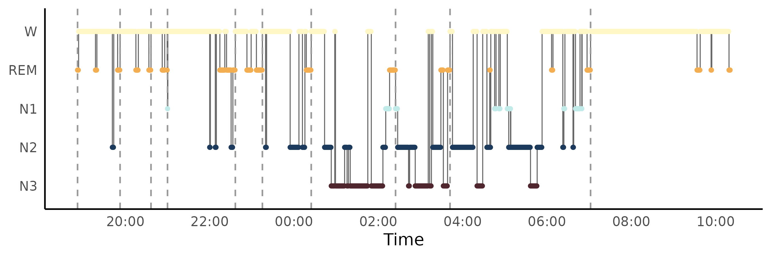

plot_hypnogram(hyp_sleep, style = "capsule")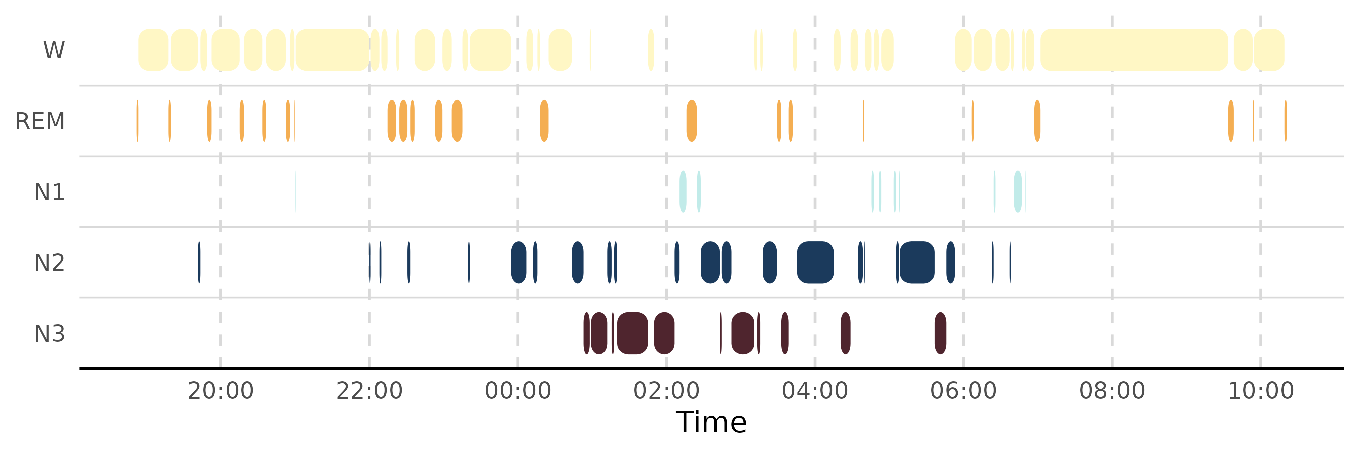

Takeaways

Scattered, brief stage flips in raw automatic staging are expected behaviour for an unsmoothed per-epoch classifier, not automatically a bug – check confidence/run-length before assuming otherwise.
Smoothing (smooth_hypnogram()) cleans up genuine single-epoch noise, but it isn’t a substitute for windowing, and pushing it too far starts deleting real short sleep events rather than noise.
Sleep architecture and cycle analyses should almost always be windowed to the actual sleep period (window_hypnogram()) before interpretation, especially for ambulatory or naturalistic recordings that include substantial pre-/post-sleep Wake.
compute_cycles()’s two methods encode a real, debatable scoring decision (interruption tolerance), not just an implementation detail – worth checking both rather than trusting one blindly.

See zeitR-integration for the same kind of worked example on the coarse, actigraphy-derived side – different staging source, different caveats (off-wrist time, multi-night windowing), but the same habit of checking rather than assuming.